
Editor’s Note: The paper on which this article is based was originally presented at the 2024 IEEE International Symposium on Electromagnetic Compatibility &
Signal/Power Integrity (EMC + SIPI), where it received recognition as the Best Symposium Paper.
Naval platforms present the most severe Electromagnetic Environment (EME) in the world, created by high-powered electromagnetic emitters such as air-search, surface-search, fire-control, and navigation radars, as well as broadband communications and electronic warfare systems. The limited space available aboard surface platforms necessitates that these high-powered electromagnetic emitters be located in proximity to other electronic/electrical systems aboard ships. Sensitive electronic equipment is typically contained within Radio Frequency (RF) reflective cavities (i.e., below-deck spaces, equipment enclosures, etc.) for protection from harsh EMEs. Communications and power cables are typically routed between enclosures within such spaces, introducing inadvertent coupling paths between cavities. Additionally, as the topside EME continues to increase and as below-deck transmitters (i.e., RFID, Wi-Fi, etc.) are incrementally installed within the Fleet, understanding and predicting the field distributions within coupled spaces will assist in characterizing electronic equipment performance and assuring personnel safety.
Statistical electromagnetic formalisms for electromagnetic fields within RF-reflective cavities had their beginnings through the study and use of reverberation chambers (RCs) for Electromagnetic Compatibility (EMC) testing [1] and are now widely accepted within the EMC community as a tool for compatibility and susceptibility testing [2-4]. RCs are electromagnetically reflective cavities with a high quality (Q) factor where the fields excited within the cavity reverberate [4-6]. The addition of tuners within the chamber (also known as paddles or stirrers) allows for the electromagnetic (EM) boundary conditions to be easily changed so the EM fields can be perturbed discretely (mode-tuned) or continuously (mode-stirred).
The statistics of RCs have been well studied and show the magnitude of a single spatial electric-field component, |Er|, will follow a chi-distribution with two degrees of freedom, and the square magnitude of this same component, |Er|2, follows a chi-square distribution with two degrees of freedom; both distributions are also widely known as the Rayleigh and exponential distribution, respectively [4, 6].
This project takes an alternative approach to the already growing interest in describing the field statistics within nested cavities [8-13]. Previous studies examined the case when two cavities are coupled via an aperture [8-9]. These studies hypothesized that the double-Rayleigh distribution would model the nested field statistics, but were unsuccessful in demonstrating it as a good fit for all test cases. This study hypothesized the same distribution but alternatively uses N wire penetrations as the coupling mechanism (vice apertures) and analyzes the statistics of the received power for each N case.
Statistical Background
Hypothesized Distributions
The chi-squared distribution with two degrees of freedom, also known as the exponential distribution and the double-Rayleigh distribution, will be considered in this study ([8] provides further background for both distributions). Because the double-Rayleigh distribution is the product of two Rayleigh random variables (RVs), which implies studying electric fields, the authors have chosen to name its power form [8] the double-exponential (DE) distribution because it implies the studying of received powers. (This distribution is not to be confused with the Laplace distribution that is sometimes referred to as a “double-exponential distribution” [14-15].) The probability density function (PDF) for the exponential distribution and double-exponential distribution is
![]() Eq. 1
Eq. 1
and
 Eq. 2
Eq. 2
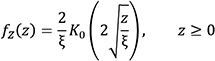
respectively, where μ is the scale parameter in (1), x = |Er|2, ξ is the scale parameter in (2), Z is the product of two independent exponential RVs (Z = XY), and KO(~) is the 0th order modified Bessel function of the second kind. See [8] for further explanation and the cumulative distribution function (CDF) of (2).
Scale Parameter Estimation and Hypothesis Testing
The scale parameter for equations (1) and (2) was estimated using the maximum likelihood estimation (MLE) method. Anderson-Darling (AD) goodness-of-fit (GOF) testing was used to assess the data against an exponential distribution and chi-squared GOF testing was used to assess the data against both an exponential distribution and the DE distribution. Detailed mechanics of MLE when applied to the exponential distribution and the DE distribution, as well as why these two GOF tests were selected are discussed in detail in [8].
Experimental Setup
Reverberant Cavities
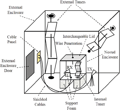
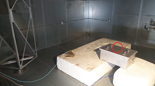
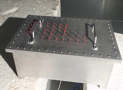
Two RCs were used in this study, one constructed of aluminum and the other constructed of zinc-coated steel. The aluminum cavity is referred to as the nested enclosure, while the zinc-coated steel cavity is referred to as the external enclosure. The physical dimensions of both enclosures are provided in Table 1. The external enclosure contains both a vertical and horizontal Z-fold tuner, while the nested enclosure contains a vertical Z-fold tuner. The nested enclosure was placed on support foam within the working volume of the external enclosure. Figures 1 and 2 provide a sketch and picture of the nested measurement setup for a single coupling antenna (N = 1). The single coupling antenna is circled in red in Figure 2.
| Dimensions | NestedCavity (meters) | ExternalCavity (meters) |
| Length | 0.70 | 5.51 |
| Width | 0.44 | 5.25 |
| Height | 0.31 | 3.56 |
Table 1: Enclosure dimensions
Measurement Setup
A Vector Network Analyzer (VNA) was used for data capture in this study. The VNA output power was set to 0 dBm, and a 150W amplifier was used to ensure all coupled measurement configurations achieved data above the VNA’s noise floor. S21 measurements were swept across the frequency range of 8 to 12 GHz at 1 MHz steps (4001 points total) with a step dwell sweep setting of 1 millisecond (ms). This frequency range ensured both enclosures were sufficiently overmoded. All three tuners (two external, one nested) were simultaneously stepped 100 times. At each step, an |S21| measurement was performed across the full frequency range, resulting in 4001 sample sets (one at each frequency), each set containing 100 independent samples.
Both enclosures were originally measured in isolation from one another to verify that both indicate exponential received power. The AD test was used to test each sample set against an exponential distribution at a 95% confidence level. The null hypothesis rejected 4.75% of the sample sets for the external enclosure and 6.15% of the sample sets for the nested enclosure, both at the defined confidence level. The rejection rates are near that of an ideally operating RC at a 95% confidence and can therefore be used for this study.
Test Cases
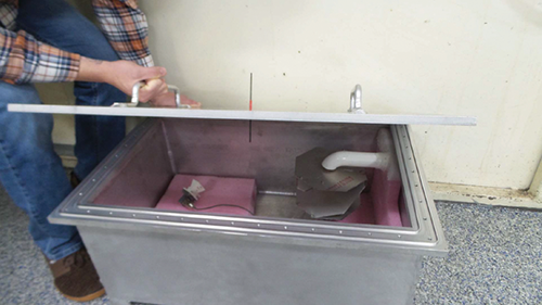
A visual representation of the nested configuration is shown in Figure 1 and a picture of the setup is shown in Figure 2. As depicted in Figure 3, a single insulated 12-gauge wire, measuring six inches in length, evenly extends externally and internally to the nested enclosure through a 3.5-millimeter (mm) hole. The wire does not make any electrical contact with the enclosure. This single wire penetration is the N = 1 test case. A total of thirty test cases were performed, each N case corresponding to the number of independent wire penetrations. The N = 1, 2, 5, 10, 15, 20, and 30 test cases are shown in this paper for brevity; Figure 4 shows the N = 30 wire penetrations, each separated by ~5-centimeters. For each test case, the total number of independent distributions tested was 4001, one for each frequency recorded. The ideal GOF test would have a 5% rejection rate at a 95% confidence (which is approximately 200 distributions rejecting the null hypothesis).
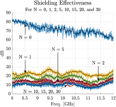
Shielding Effectiveness
The nested enclosure’s shielding effectiveness (SE) was measured following the procedures in [16] and is shown in Figure 5. The nested enclosure was measured to show approximately 80 dB of SE at the lower frequencies, which reduces to 60 dB SE at the higher frequencies over the frequency range of this study (N = 0 configuration). The other seven test cases are also shown in Figure 5, and it shows the SE significantly reduces for the N = 1 wire penetration, and as more wire penetrations are added the impact of the reduction in SE reduces eventually reaching a point of diminishing returns, i.e., the two enclosures were acting as a single enclosure. The black line for each test case represents a 50MHz smoothing to emphasize the trend the SE follows for each test case.
De Gof Results
Table 2 shows the total percentage of values that rejected the null hypothesis in GOF testing, where each column represents the associated distribution and respective GOF test. All GOF testing was used to test the data against the respective hypothesized distribution at a 95% confidence. Data tested against an exponential distribution using the AD test and the chi-square GOF test are represented by EX-AD and EX-χ2, and data tested against the DE distribution using the chi-square GOF test is represented by the DE-χ2.
| Test Case N | Percentage of Rejected Distributions Tested at a95% Confidence Value | ||
| EX–AD | EX–χ2 | DE–χ2 | |
| 1 | 99.90 % | 97.30 % | 5.52 % |
| 2 | 89.85 % | 56.46 % | 24.29 % |
| 5 | 39.04 % | 14.55 % | 63.06 % |
| 10 | 13.72 % | 6.57 % | 79.76 % |
| 15 | 9.92 % | 6.92 % | 84.68 % |
| 20 | 7.50 % | 6.65 % | 86.50 % |
| 30 | 6.52 % | 6.35 % | 88.25 % |
Table 2: Percentage of exponential and DE distributions that rejected the null hypothesis at a 95% confidence
For the N = 1 case, the exponential distribution is almost entirely rejected for both the AD and chi-square GOF tests, with the total amount rejecting the null hypothesis being 99.90% and 97.30%, respectively. However, the total amount of distributions that rejected the DE distribution was 5.52%, strongly indicating that the DE provides a good fit for the data in this specific test case.
For the N = 2 and 5 cases, the exponential distribution is rejected decreasingly less than the N = 1 case, but still at too great a rate for evidence of an exponential distribution. However, comparing the N = 2 and 5 cases, it is becoming evident that fewer distributions can reject the null hypothesis when tested against the exponential distribution. Additionally, it should not be surprising that the AD and chi-square GOF rejections are different, with the chi-square being less powerful than the AD test, as shown in [23]. The rejection rate for the DE distribution demonstrates the exact opposite trend as the exponential distribution, with more distributions being rejected as the number of independent wire penetrations increases.
As N continues to increase, the evidence of the exponential distribution increases to where finally the two GOF tests have near identical total rejected values (i.e., N = 30 test case). For the N ≥ 20 test cases, the two enclosures are statistically operating as a single RC. Alternatively, the DE distribution only provides a good fit for a single wire penetration (i.e., N = 1) and is rejected for all other test cases (i.e., N > 1).
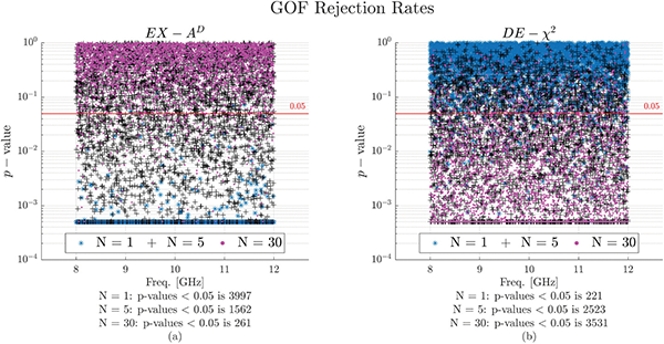
The transitions in GOF rejection rates are visually depicted in Figure 6. As N increases for the exponential distribution, the total number of rejected values decreases, as seen in Figure 6a for the AD GOF tests, while the total number of rejected values increases for the DE distribution using the chi-square GOF test shown in Figure 6b.
N-Coupled Cavity Hypothesis
We have shown that for a single wire penetration between nested enclosures, the received power closely follows the DE distribution. However, as N coupling mechanisms increase, the DE is no longer suitable to describe the distribution of the fields, and the exponential distribution only begins to confidently describe the fields for sufficiently high N cases. We now examine the potential for a new hypothesized distribution to be able to describe this transitional region between the two extremes (i.e., 1 < N < 30).
Taking a step back and conceptually understanding what is going on under the lid, each new coupling mechanism (i.e., wire penetration) is introducing an independent exponential RV into the nested enclosure. Since each wire penetration is introducing power into the nested enclosure through the coupled power from the exposed wire within the external enclosure, each exponential RV is from the same parent distribution, specifically the external chamber’s exponential distribution. Additionally, when sufficiently spaced (by at least λ /4 to ensure spatially uncorrelated samples), each wire penetration introduces an independent, identically distributed (IID) RV.
The Erlang Distribution
Based on the characteristics of the physical mechanics of the electromagnetic fields within the nested enclosure, one may predict that the distribution of the total power coupled into the nested enclosure from the external enclosure may be sufficiently described by the sum of N IID exponential distributions, or equivalently the Erlang distribution [17-18]. The Erlang distribution is a special case of the gamma distribution, specifically for positive integer values of N [18-19], and the PDF of the Erlang distribution is defined as
![]() Eq. 3
Eq. 3
where W = ∑NXN (the sum of N IID exponential RVs), N is an integer, and σ is the scale parameter (σ = 1/λ in [18], where λ is the rate parameter).
Nested Enclosure Hypothesized Distribution for N ≥ 1
With the total power introduced into the nested enclosure defined by the Erlang distribution, following the same principles defined in [8], the distribution of the nested cavity is defined as the product of the Erlang RV (W) and the nested enclosure’s exponential RV (Y)
![]() Eq. 4
Eq. 4
where Z’ is the RV of a distribution the authors have termed the modified-Double Exponential (MDE) distribution. By invoking a statistical theorem for the product of two independent RVs [20],
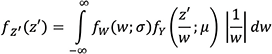 Eq. 5
Eq. 5
where f(w; σ) and (inline equation) represent the Erlang and exponential distributions, respectively. We derive the PDF of the MDE through leveraging 3.471.9 in [21], and changing the lower bound in (5) to 0 because all variables are positive values.
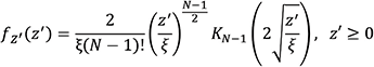 Eq. 6
Eq. 6
where ξ is the scale parameter and ξ > 0. The MDE CDF is then calculated through the integration of the PDF, or specifically,
 Eq. 7
Eq. 7
In the specific case of one independent wire penetration (i.e., N = 1), it is easily shown that the PDF and CDF of the MDE reduce to the DE PDF in (2) and CDF in [8]. By employing MLE to estimate the MDE parameter ξ, the log likelihood function is derived to be (8), and the same numerical approach described in [8] was used to estimate the scale parameter ξ.
MDE GOF Test Results
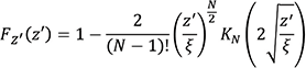
The chi-square GOF test is again used to test the data against the hypothesized MDE distribution at a 95% confidence for all N test cases. Table 3 repeats the data in Table 2 with a new column, identified by MDE-χ2, reflecting the percentage of distributions that rejected the null hypothesis at the 95% confidence for the hypothesized MDE distribution using the chi-square GOF test. For all N test cases, the chi-square GOF test rejects the null hypothesis at a near-ideal rejection rate. This indicates that the MDE distribution provides a good fit when describing the statistics of received power within the nested enclosure for all quantities of wire penetrations tested. Figure 7 shows the p-values for the N = 1, 5, and 30 test cases and the total number of p-values below 0.05, further emphasizing that the MDE distribution is a good fit to the experimental data.
| Test Case N | Percentage of Rejected Distributions Tested at a 95% Confidence Value | |||
| EX–AD | EX–χ2 | DE–χ2 | MDE–χ2 | |
| 1 | 99.90% | 97.30% | 5.52% | 5.52% |
| 2 | 89.85% | 56.46% | 24.29% | 5.45% |
| 5 | 39.04% | 14.55% | 63.06% | 5.97% |
| 10 | 13.72% | 6.57% | 79.76% | 5.50% |
| 15 | 9.92% | 6.92% | 84.68% | 6.12% |
| 20 | 7.50% | 6.65% | 86.50% | 6.17% |
| 30 | 6.52% | 6.35% | 88.25% | 5.62% |
Table 3: Percentage of MDE distributions that rejected the null hypothesis at a 95% confidence level
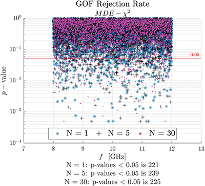
For the N = 30 test case, it is interesting that both the exponential and MDE provide a good fit to the experimental data. The authors intuitively interpret this result from the following: for large N, the Erlang distribution converges to a Normal distribution by the Central Limit Theorem [20]. (In [11], the authors reach a similar conclusion for “the case of many apertures.”) Additionally, by the Law of Large Numbers, the variance of the Normal distribution approaches zero with increasing N [18, 20], or equivalently approaches a Dirac delta function (a constant) [24]. Figure 8 illustrates both the mean normalized Erlang distribution converging to a Normal distribution and the variance of the Normal distribution decreasing with increasing N for theoretical mean normalized data. Therefore, for large N, (4) approaches the product of a “constant” and the exponentially distributed random variable of the nested enclosure, or simply a scaled exponential distribution.
The authors recognize that the derivation of the MDE (and DE) does not account for energy returning to the external enclosure through the wire penetration(s). Hence, the MDE may not sufficiently describe the statistics for all enclosure/coupling configurations. For example, at lower frequencies where the wall losses are less dominant than antennas [6] more energy may be exchanged between the external and nested enclosures through various coupling mechanisms. Therefore, the authors are working to derive a distribution by applying a conservation of energy approach similar to [22], which was done for averages.
 Eq. 8
Eq. 8
Conclusion
A study has been performed in which two analyses have been completed to characterize the statistical distribution of a nested enclosure when coupled by N wire penetrations. Mode tuning was utilized to simultaneously perturb the electromagnetic environments in both external and nested enclosures. Both enclosures were first shown to exhibit exponentially distributed received power when tuned in isolation. Appropriate and rigorous statistical tests were used to evaluate the GOF for three hypothesized distributions: the exponential, DE, and MDE distributions.
The DE distribution provided a good fit when the two enclosures were coupled by a single wire penetration (N = 1). For the N > 1 cases, non-DE behavior was observed. The characteristics of an exponential distribution became evident as a large number of wire penetrations (N ≥ 20) were implemented on the enclosure. For N < 20 wire penetrations, the disagreement between the rejection rates of the AD and chi-square GOF tests against the exponential was too different and too large to suggest that exponential behavior is present at the 95% confidence level.
The MDE distribution was then introduced and shown to have a good fit for all test cases (1 ≤ N ≤ 30), indicating it is a good distribution to choose when characterizing the received power under the conditions present in this experiment. Further work will be done to analyze nested enclosures when energy balance [22] is taken into consideration, as well as when apertures are used as test cases.
References
- H. A. Mendes, “A new approach to electromagnetic field-strength measurements in shielded enclosures,” Wescon, Los Angeles, CA, 1986.
- IEC 61000-4-21 Electromagnetic Compatibility: Reverberation Chamber Test Methods, International Electrotechnical Commission (IEC), Geneva, Switzerland, August 2003.
- MIL-STD-461G: Requirements for the Control of Electromagnetic Interference Characteristics of Subsystems and Equipment, US DoD Interface Standard, 11 December 2015.
- D.A. Hill, Electromagnetic Fields in Cavities: Deterministic and Statistical Theories, Wiley-IEEE Press, 2009.
- R. Serra et al., “Reverberation chambers a la carte: An overview of the different mode-stirring techniques,” IEEE Electromagnetic Compatibility Magazine, vol. 6, no. 1, pp. 63-78, 2017.
- D. A. Hill, Electromagnetic Theory of Reverberation Chambers (NIST Technical Note 1506). Gaithersburg, MD, U.S. Department of Commerce, National Institute of Standards and Technology, 1998.
- M. L. Crawford and G. H. Koepke, Design, evaluation, and use of a reverberation chamber for performing electromagnetic susceptibility/vulnerability measurements (NBS Technical Note 1092), Gaithersburg, MD, U.S. Dept. of Commerce, National Bureau of Standards, 1986.
- M. D. Sowell and J. C. West, “Statistics of Electromagnetic Fields within Aperture-Coupled, Nested Reverberant Cavities,” IEEE Symposium on Electromagnetic Compatibility, Grand Rapids, MI, July 2023.
- Y. He and A. C. Marvin, “Aspects of field statistics inside nested frequency-stirred reverberation chambers,” IEEE International Symposium on Electromagnetic Compatibility, Austin, TX, August 2009, pp. 171-176.
- C. E. Hager IV and G.B. Tait, “Maximum Received Power Statistics within RF Reflective Enclosures for HERO/EMV Testing,” IEEE Symposium on Electromagnetic Compatibility, Santa Clara, CA, March 2015, pp. 237-241.
- M. Höijer and L. Kroon, “Field Statistics in Nested Reverberation Chambers,” IEEE Transactions on Electromagnetic Compatibility, vol. 55, no. 6, pp. 1328-1330, December 2013.
- G. Gradoni, J. -H. Yeh, T. M. Antonsen, S. Anlage, and E. Ott, “Wave chaotic analysis of weakly coupled reverberation chambers,” IEEE International Symposium on Electromagnetic Compatibility, Long Beach, CA, 2011, pp. 202-207.
- W. Qi et al., “Statistical Analysis for Shielding Effectiveness Measurement of Materials Using Reverberation Chambers,” IEEE Transactions on Electromagnetic Compatibility, vol. 65, no. 1, pp. 17‑27, Feb. 2023.
- Marco Geraci and Mario Cortina Borja, “Notebook: The Laplace Distribution,” Significance, vol. 15, no. 5, October 2018, pp. 10-11.
- H. I. Okagbue et al, “Laplace Distribution: Ordinary Differential Equations,” World Congress on Engineering and Computer Science, San Francisco, CA, October 2018.
- C. L. Holloway et al., “Use of Reverberation Chambers to Determine the Shielding Effectiveness of Physically Small Electrically Large Enclosures and Cavities,” IEEE Transactions on Electromagnetic Compatibility, vol. 50, no. 4, pp. 770-782, 2008.
- W. K. Grassmann, “Computational Methods in Probability Theory,” Stochastic Models, vol. 2, Edited by D. P. Heyman and M. J. Sobel, Elsevier Science Publishers B.V., 1990., Ch. 5, sec 2.8, pp. 221-223.
- S. Kay, Intuitive Probability and Random Processes using MATLAB®, New York, NY, Springer, 2006.
- S. Miller and D. Childers, “Random Variables, Distributions, and Density Functions,” Probability and Random Processes: With Applications to Signal Processing and Communications, 2nd ed., Waltham, MA, USA: Academic Press, 2012, ch. 3, sec. 3.4.5, pp. 81‑82
- P. L. Meyer, Introductory Probability and Statistical Applications, 2nd ed., Reading, MA, USA: Addison-Wesley Pub. Co., 1970.
- I.S. Gradshteyn and I. M. Ryzhik, “Definite Integral of Elementary Functions,” Table of Integrals, Series, and Products, 8th ed, Waltham, MA, Academic Press, 2014, Ch. 3, section 3.471, pp. 370.
- G. B. Tait, R. E. Richardson, M. B. Slocum, M. O. Hatfield, and M. J. Rodriguez, “Reverberant Microwave Propagation in Coupled Complex Cavities,” IEEE Transactions on Electromagnetic Compatibility, February 2011, vol. 53, no. 1, pp. 229-232.
- A. O. Lima et al, “Extreme Rainfall Events Over Rio de Janeiro State, Brazil: Characterization Using Probability Distribution Functions and Clustering Analysis,” Atmospheric Research, vol. 247, 2021.
- J. Lie and J. Chen, Stochastic Dynamics of Structures, John Wiley & Sons (Asia) Pte Ltd, 2009.